Part 1: Imitation Learning & Why It Breaks
RL to RLHF — A Practitioner's Guide to Deep RL Part 1 of 8
What if the simplest approach to teaching an AI — just showing it what to do — has a fatal flaw baked into its design?
That approach is called Behavioral Cloning, and if you've heard of Supervised Fine-Tuning (SFT) for large language models, you already know it. Same algorithm, same math, same failure mode.
This post walks through both the method and the flaw, with from-scratch implementations that make the problem visible.
Introduction
Most machine learning you've seen is supervised — you have inputs, labels, and you minimize a loss function. Reinforcement Learning (RL) is fundamentally different. There are no labels. Instead, an agent takes actions in an environment, receives rewards, and must figure out — on its own — what sequence of actions maximizes total reward. But what if we could skip the hard part? What if we just watched an expert and copied what they did? That's the idea behind Behavioral Cloning (BC) — and it works surprisingly well. Until it doesn't. In this post, we'll build BC from scratch, watch it fail in a spectacular and instructive way, and then fix it with a clever algorithm called DAgger. Everything we build here maps directly to how Large Language Models are trained: Supervised Fine-Tuning (SFT) is literally Behavioral Cloning applied to text. Understanding why BC fails with a walking robot makes it obvious why SFT alone isn't enough for ChatGPT.
Section 1: What Is Reinforcement Learning?
In RL, an agent interacts with an environment in a loop:
The agent observes the current state
It picks an action
The environment responds with a new state and a reward
Repeat
The goal: find a policy (a strategy for choosing actions) that maximizes total reward over time.
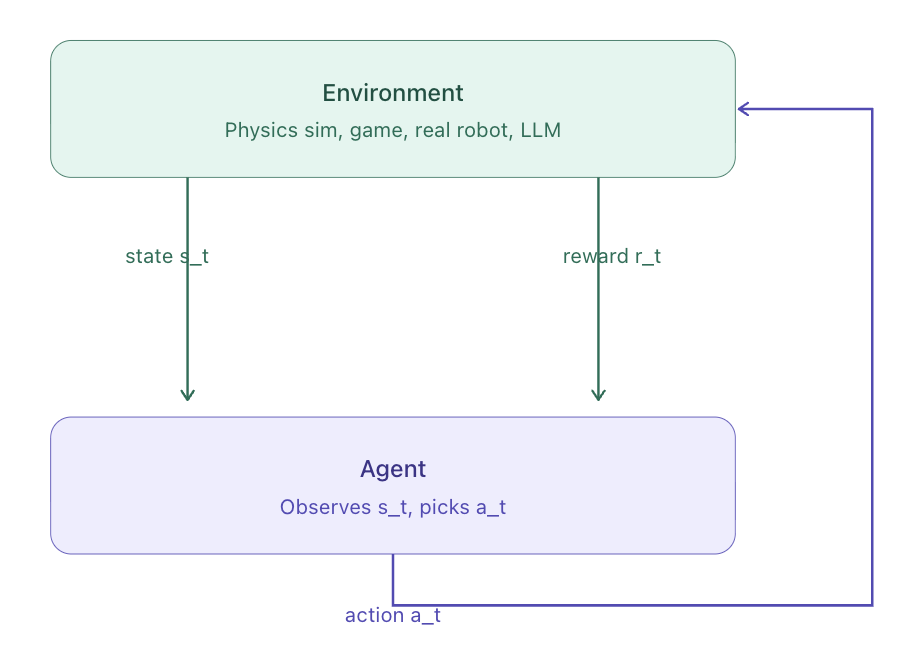
Figure 1: The Reinforcement Learning loop. At each time step, the agent observes the current state s_t, from the environment, takes an action a_t, and in return receives a new state and a reward r_t.
Why is this hard?
Rewards are sparse — you might only know an action was good long after you took it (like chess, where the reward comes at the end of the game)
Actions have long-range consequences — step 1 affects what happens at step 1000
The agent must balance exploration (trying new things) vs exploitation (doing what worked before)
💡 The LLM Connection: When you fine-tune a language model on human-written responses, you're doing behavioral cloning. The prompt is the state, the human response is the expert action, and cross-entropy is the loss. This stage is called SFT (Supervised Fine-Tuning), and it's step 1 of how ChatGPT was trained.
Section 2: The MDP — Formalizing Decision-Making
To reason rigorously about RL, we use the Markov Decision Process (MDP) framework.
An MDP has five components:
| Symbol | Name | Meaning |
|---|---|---|
| S | State space | Everything the agent can observe |
| A | Action space | Everything the agent can do |
| P(s'|s,a) | Transition function | How the world changes given state + action |
| R(s,a) | Reward function | Scalar feedback signal |
| γ ∈ [0,1) | Discount factor | How much we value future rewards |
The Markov property makes this tractable: the next state depends only on the current state and action, not on the full history.
A policy π(a|s) tells the agent what action to take in each state. The goal of RL is to find the optimal policy π* that maximizes the expected discounted return:
The discount factor γ means a reward of +1 now is worth more than +1 later. At γ=0.99, a reward 100 steps away is worth about 37% of an immediate reward.
Section 3: The Ant-v5 Environment
We work with Ant-v5 from MuJoCo — a physics simulator widely used in RL research. The ant is a 3D quadruped robot.
The task: walk forward as fast as possible without falling.
This is a continuous control task — unlike games where you press buttons, the ant's joints require precise, real-valued torques. This makes it a useful proxy for both robotics and, conceptually, for language models (which also produce continuous-valued distributions over tokens).
Figure 2: The expert SAC policy walking the Ant-v5 robot. This is our gold standard — the behavior we want to imitate.
Why Ant-v5 for this series?
- Continuous actions — forces us to use regression, not classification
- High-dimensional state (27 dimensions) — distribution shift is actually visible, not hidden by problem simplicity
- Non-trivial dynamics — the ant can fall in infinitely many ways; recovery matters
- Standard benchmark — directly comparable to published results
The MDP for Ant-v5:
| Component | Details |
|---|---|
| State | 27D continuous vector (joint angles, velocities, torso pose) |
| Action | 8D continuous torques, one per joint, clipped to [-1, 1] |
| Reward | forward_velocity − control_cost − unhealthy_penalty |
| Episode end | Ant falls (height < 0.2 or > 1.0) or 1000 steps reached |
A random policy — just applying random torques — scores about -50 to +200 reward and the ant falls almost immediately. A good policy should reach 4000–8000+ reward.
Section 4: Behavioral Cloning — Learning by Imitation
Suppose we have an expert that already knows how to walk. Instead of figuring out the reward signal ourselves, can we just copy what the expert does?
Behavioral Cloning (BC) does exactly this:
Watch the expert → collect (state, action) pairs
Train a neural net to predict the expert's action from the state
Deploy the trained net as our policy
That's it. BC is just supervised learning — the state is the input, the expert's action is the label.
For continuous actions like joint torques, we minimize the mean squared error (MSE) between predicted and expert actions. An MSE of 0.01 means the policy is off by about 0.1 torque units per joint — pretty accurate.
💡 The LLM connection: Supervised Fine-Tuning (SFT) — the first stage of ChatGPT training — is exactly BC. The "expert" is a human writer, the "state" is the prompt, and the "action" is the next token. Training maximizes likelihood of the human's tokens — same as minimizing loss on expert demonstrations.
The Expert
We use a pretrained SAC (Soft Actor-Critic) model from HuggingFace Hub. SAC is an RL algorithm trained purely from the environment's reward signal — no demonstrations needed. It's our gold standard.
Just like you'd load `bert-base-uncased` for NLP, the RL community shares pretrained policies on HuggingFace.
The Policy Network
A simple 3-layer MLP maps observations to actions:
class PolicyNet(nn.Module):
    def __init__(self, obs_dim, action_dim, hidden=256):
        super().__init__()
        self.net = nn.Sequential(
            nn.Linear(obs_dim, hidden), nn.ReLU(),
            nn.Linear(hidden, hidden),  nn.ReLU(),
            nn.Linear(hidden, action_dim), nn.Tanh(),  # Tanh keeps outputs in [-1, 1]
        )

    def forward(self, x):
        return self.net(x)
Why Tanh on the output? Ant-v5 motor torques are bounded to [-1, 1]. Without Tanh, the network could output 100.0 — the environment clips it, but the gradient of a clipped value is zero. The network would receive no learning signal. Tanh keeps everything in range smoothly.
Training BC
We collect 50 expert episodes (~50,000 state-action pairs), then train with standard supervised learning:
# Collect expert demonstrations
demo_obs, demo_actions = collect_demonstrations(expert.predict, n_episodes=50)
# Dataset: 50,000 transitions

# Train: minimize MSE between predicted and expert actions
policy = PolicyNet(obs_dim=27, action_dim=8)
optimizer = Adam(policy.parameters(), lr=1e-3)

for epoch in range(100):
    for obs_batch, action_batch in dataloader:
        loss = mse_loss(policy(obs_batch), action_batch)
        optimizer.zero_grad()
        loss.backward()
        optimizer.step()
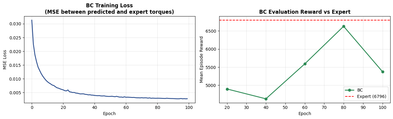
BC training loss (MSE) dropping over 100 epochs. Lower means the policy's predictions are closer to the expert's actions.
BC achieves roughly 60 - 80% of the expert's reward. Not terrible — but clearly something is wrong.
Section 5: Distribution Shift — The Fatal Flaw
The Problem
BC trains on states the expert visits. But at test time, the learned policy makes slightly different decisions, visiting slightly different states — states it has never seen during training.
Training time:
- Expert always walks centered and balanced
- Dataset only contains balanced-ant states
- Policy learns: "when balanced → keep walking"
Test time:
- Tiny prediction error → ant leans slightly left
- Policy has NEVER seen a leaning-left state
- Doesn't know how to correct → lean gets worse → more unseen states → falls
This gap between the training state distribution and the test-time state distribution is called distribution shift.
Compounding Errors
If the per-step error rate is ε, the total error after T steps is proportional to ε × T² — quadratic in episode length. For a 1000-step Ant episode, this is catastrophic.
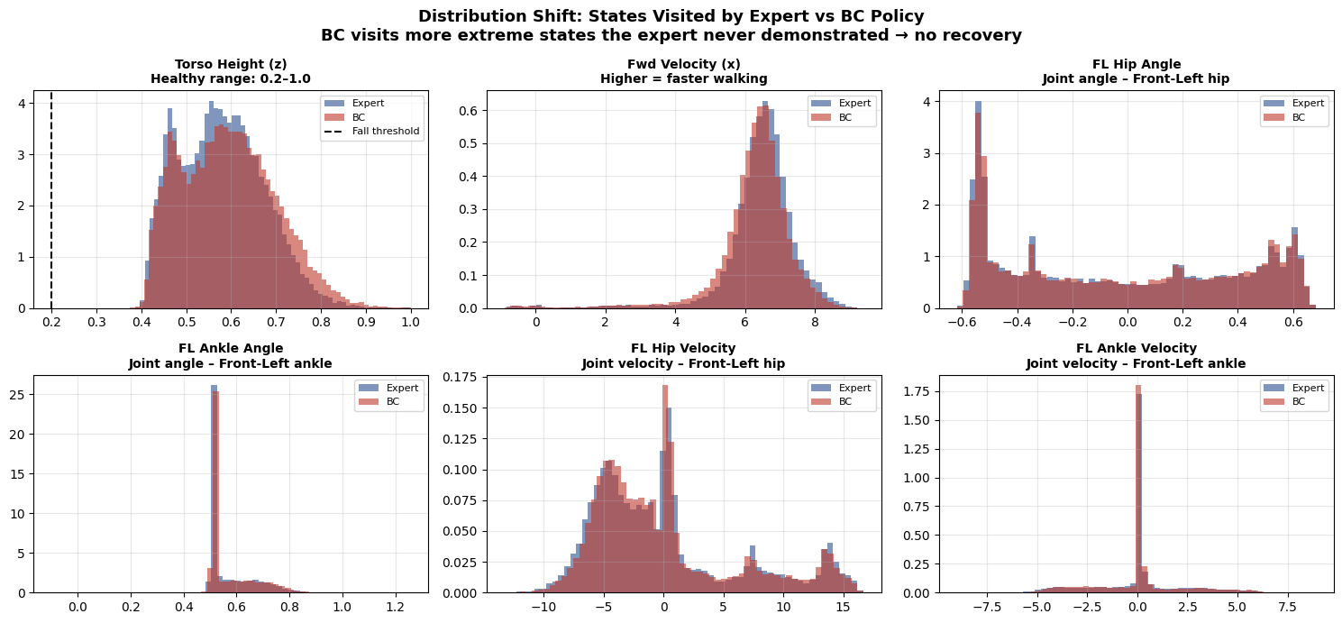
Expert is maintaining stable height around 0.6(lower compare to BC) and able to walk faster compare to BC.
Section 6: DAgger — Fixing Distribution Shift
DAgger (Dataset Aggregation, [Ross et al. 2011](https://arxiv.org/abs/1011.0686)) fixes the problem by changing which states we collect training data on.
The Algorithm
1. Collect initial dataset D from expert rollouts
2. Train policy π on D
3. Repeat:
- a. Roll out π (the learner, not the expert) → collect the states the learner visits
- b. Ask the expert: "what would YOU do in each of these states?"
- c. Add (learner_state, expert_action) pairs to D
- d. Retrain π on the full, growing D
Why It Works
The key insight: we collect data where the learner goes, not where the expert goes.
- Iteration 1: D = only expert states. Policy walks okay but wobbles.
- Iteration 2: Policy wobbles → visits wobbly states → expert labels those → D now contains recovery examples.
- Iteration 3: Policy is more stable → explores slightly further off-balance states → expert labels those too.
- After N iterations: D covers both expert states AND all the states the learner tends to visit. No more unknown territory.
Concrete Example for Ant-v5
Think about what happens at each DAgger iteration:
Iter 1: The ant wobbles and its front-left hip angle reaches 0.42 (outside the expert's usual range). The expert is asked "what would you do here?" and says: "apply -0.3 torque to correct." This (wobble_state, correction_action) pair enters the dataset.
Iter 2: The policy has now seen recovery examples. It wobbles less but encounters new edge cases. The expert labels those too.
Iter N: The policy can recover from almost any perturbation it's likely to encounter.
Theoretical Guarantee
| Algorithm | Error Bound |
|---|---|
| BC | O(ε × T²) — quadratic in episode length |
| DAgger | O(ε × T) — linear in episode length |
For T=1000 (Ant episode), DAgger has up to 1000× smaller worst-case error.
def train_dagger(expert_predict_fn, n_iterations=10):
    # Step 1: seed with expert rollouts
    D_obs, D_actions = collect_expert_demos(n_episodes=10)

    for it in range(n_iterations):
        # Step 2: train policy on aggregated dataset
        policy = train_on_dataset(D_obs, D_actions)

        # Step 3: roll out LEARNER, label with EXPERT
        for episode in range(10):
            obs = env.reset()
            while not done:
                learner_action = policy.predict(obs)     # learner acts
                expert_action  = expert.predict(obs)     # expert labels
                D_obs.append(obs)
                D_actions.append(expert_action)          # store expert's label!
                obs, _, done, _ = env.step(learner_action)

    return policy
The Catch — Expert Query Cost
Every DAgger iteration queries the expert on new states. If the expert is a pretrained model (like our SAC agent), this is cheap. But if the expert is a human labeler, it gets expensive fast.
This cost is exactly what motivates RLHF (Part 7): instead of querying humans on every state, we train a reward model that predicts human preferences, and use RL to optimize against it. One-time labeling cost, unlimited training.
Section 7: Results — BC vs DAgger vs Expert
Let's see how everything stacks up:
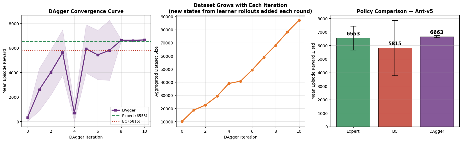
Full comparison: DAgger progressively closes the gap with the expert as it aggregates more data.
| Algorithm | Mean Reward | % of Expert | Key Limitation |
|---|---|---|---|
| Random | ~100 | ~1% | No learning at all |
| BC | ~4000–6000 | ~50–70% | Distribution shift — falls in unseen states |
| DAgger | ~6000–7000 | ~70–90% | Needs expert access at every iteration |
| Expert (SAC) | ~7000–8000 | 100% | Trained with RL from scratch (expensive) |
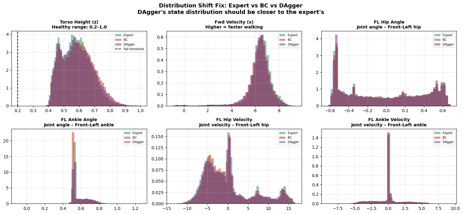
DAgger closes the distribution gap. Its state distribution (purple) is much closer to the expert's (blue) than BC's was (red).
Section 8: Summary & What's Next
What We Built
| Algorithm | Core Idea | Failure Mode | Error Bound |
|---|---|---|---|
| BC | Supervised learning on expert (state, action) pairs | Distribution shift — falls in states never demonstrated | O(ε T²) |
| DAgger | Aggregate expert labels on learner states | Needs expert at every iteration (cost) | O(ε T) |
The Bridge to LLMs
| RL Concept | LLM Equivalent |
|---|---|
| State | Prompt + generated tokens so far |
| Action | Next token |
| Expert | Human writer |
| BC | Supervised Fine-Tuning (SFT) |
| DAgger | Interactive human-in-the-loop training |
| Expert query cost | Human labeling cost → motivates RLHF |
What's Next
BC and DAgger both need an expert. In Part 2, we remove that dependency entirely with Policy Gradients — learning directly from the environment's reward signal. No expert. No demonstrations. Just trial, error, and calculus.
Policy gradients are the foundation of PPO, which is the algorithm behind RLHF. Part 2 builds every piece from scratch.
Block: [TEXT] — Footer / CTA
Full notebook with runnable code: GitHub
Next in the series: Part 2 — Policy Gradients: Learning from Rewards